US Annual Total Natural Gas Consumption

The dataset provides information on the US annual natural gas consumption by state level between 1997 and 2019, and aggregate level between 1949 and 2019

Units: Million Cubic Feet

us_total

Format

A data.frame with 3 variables.

year

An integer, the year of the observation

state

A character, the US state indicator

y

A numeric, the yearly total natural gas consumption in a million cubic feet by state or US aggregate

Source

US Energy Information Administration (EIA) website.

Details

The dataset contains a summary of the total annual demand for natural gas in the US by state and total aggregate level. The data is available for the state level between 1997 and 2019, and for the US level between 1949 and 2019.

Examples

data("us_total")

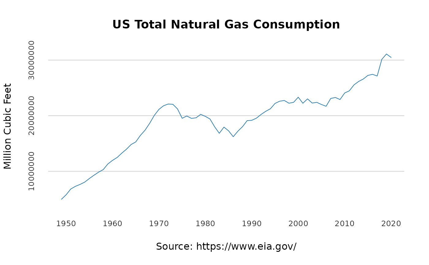
# Subsetting the total consumption in the US
us_agg <- us_total[which(us_total$state == "U.S."),]

us_agg <- us_agg[order(us_agg$year), ]

head(us_agg)
#>      year state       y
#> 1034 1949  U.S. 4971152
#> 1035 1950  U.S. 5766542
#> 1036 1951  U.S. 6810162
#> 1037 1952  U.S. 7294320
#> 1038 1953  U.S. 7639270
#> 1039 1954  U.S. 8048504

at_x <- seq(from = 1950,
            to = 2020,
            by = 10)

at_y <- pretty(us_agg$y)[c(3, 5, 7)]

plot(us_agg$year, us_agg$y,
     col = "#1f77b4",
     type = "l",
     frame.plot = FALSE,
     axes = FALSE,
     panel.first = abline(h = at_y, col = "grey80"),
     main = "US Total Natural Gas Consumption",
     xlab = "Source: https://www.eia.gov/",
     ylab = "Million Cubic Feet")



mtext(side =1, text = format(at_x,  nsmall=0), at = at_x,
      col = "grey20", line = 1, cex = 0.8)

mtext(side =2, text = format(at_y, scientific = FALSE), at = at_y,
      col = "grey20", line = 1, cex = 0.8)


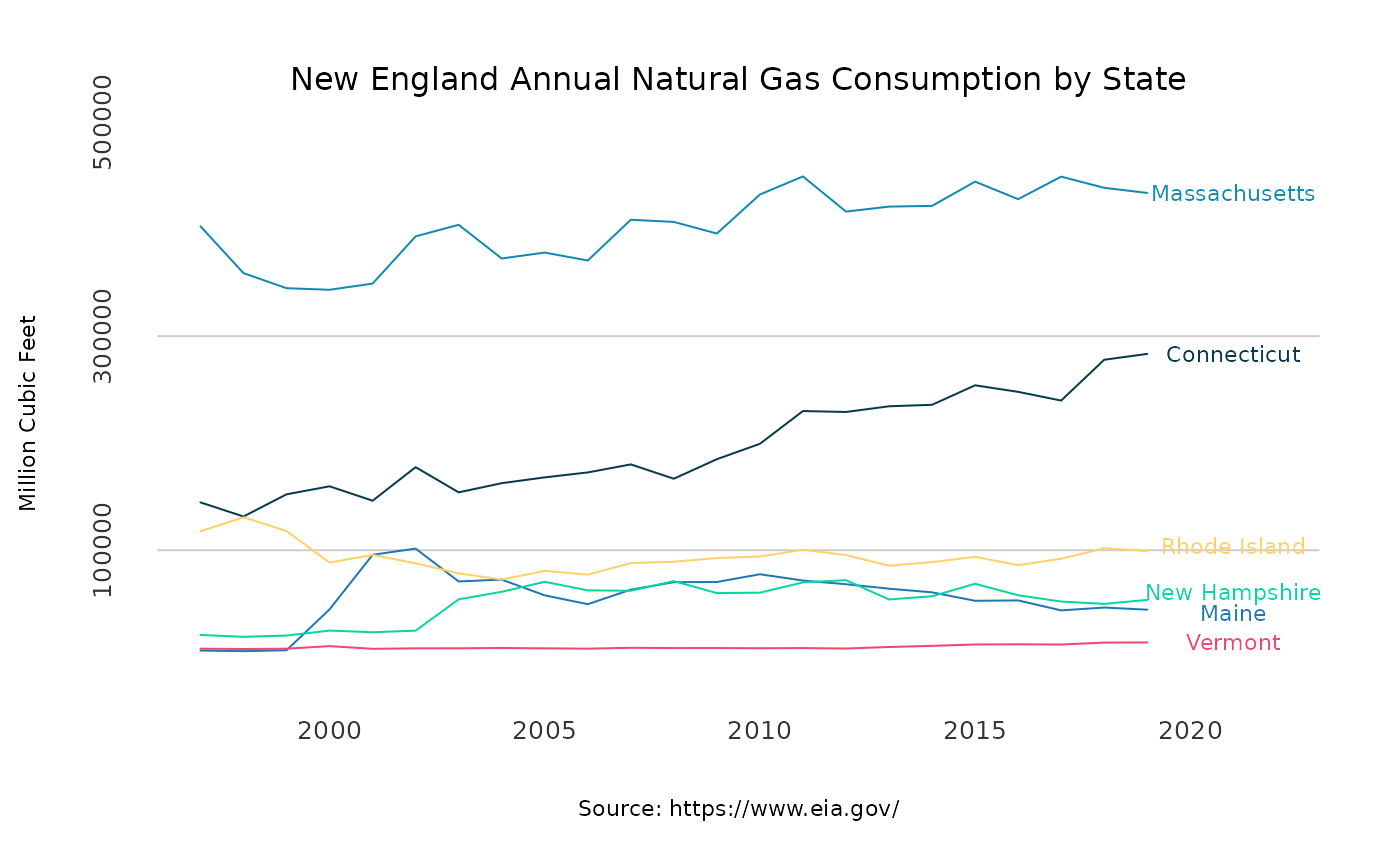
### Plotting the annual consumption in New England states
# Subsetting the New England states
ne <- c("Connecticut", "Maine", "Massachusetts",
        "New Hampshire", "Rhode Island", "Vermont")
ne_gas <-  us_total[which(us_total$state %in% ne),]

# Reshape to wide
ne_wide <- reshape(ne_gas, v.names = "y", idvar = "year",
                   timevar = "state", direction = "wide")

names(ne_wide) <- c("year",ne)
# Reorder the data
ne_wide <- ne_wide[order(ne_wide$year), ]

# Set the plot y and x axis ticks
at_x <- seq(from = 2000,
            to = 2020,
            by = 5)

at_y <- pretty(ne_gas$y)[c(2, 4, 6)]

# plot the first series
plot(ne_wide$year, ne_wide$Connecticut,
     type = "l",
     col = "#073b4c",
     frame.plot = FALSE,
     axes = FALSE,
     panel.first = abline(h = c(at_y), col = "grey80"),
     main = "New England Annual Natural Gas Consumption by State",
     cex.main = 1, font.main = 1, col.main = "black",
     xlab = "Source: https://www.eia.gov/",
     font.axis = 1, cex.lab= 0.7,
     ylab = "Million Cubic Feet",
     ylim = c(min(ne_gas$y, na.rm = TRUE), max(ne_gas$y, na.rm = TRUE)),
     xlim = c(min(ne_gas$year), max(ne_gas$year) + 3))

# Add the 5 other series
lines(ne_wide$year, ne_wide$Maine, col = "#1f77b4")
lines(ne_wide$year, ne_wide$Massachusetts, col = "#118ab2")
lines(ne_wide$year, ne_wide$`New Hampshire`, col = "#06d6a0")
lines(ne_wide$year, ne_wide$`Rhode Island`, col = "#ffd166")
lines(ne_wide$year, ne_wide$Vermont, col = "#ef476f")

# Add the y and x axis ticks
mtext(side =1, text = format(at_x, nsmall=0), at = at_x,
      col = "grey20", line = 1, cex = 0.8)

mtext(side =2, text = format(at_y, scientific = FALSE), at = at_y,
      col = "grey20", line = 1, cex = 0.8)


text(max(ne_wide$year) + 2,
     tail(ne_wide$Connecticut,1),
     "Connecticut",
     col = "#073b4c",
     cex = 0.7)

text(max(ne_wide$year) + 2,
     tail(ne_wide$Maine,1) * 0.95,
     "Maine",
     col = "#1f77b4",
     cex = 0.7)

text(max(ne_wide$year) + 2,
     tail(ne_wide$Massachusetts,1),
     "Massachusetts",
     col = "#118ab2",
     cex = 0.7)

text(max(ne_wide$year) + 2,
     tail(ne_wide$`New Hampshire`,1) * 1.1,
     "New Hampshire",
     col = "#06d6a0",
     cex = 0.7)

text(max(ne_wide$year) + 2,
     tail(ne_wide$`Rhode Island`,1) * 1.05,
     "Rhode Island",
     col = "#ffd166",
     cex = 0.7)

text(max(ne_wide$year) + 2,
     tail(ne_wide$Vermont,1),
     "Vermont",
     col = "#ef476f",
     cex = 0.7)