Data Prep

This document provides the steps of loading a dataset from a CSV file and reformating it to a time series object following Nixtla format. This includes the following steps:

• Loading the raw data from a CSV file
• Reformat the data
• Filter the data by time range

Data

We will use a preload dataset of the US hourly demand for electricity sourced from the EIA API.

The header of the query from the EIA API:

{
    "frequency": "hourly",
    "data": [
        "value"
    ],
    "facets": {
        "respondent": [
            "US48"
        ],
        "type": [
            "D"
        ]
    },
    "start": null,
    "end": null,
    "sort": [
        {
            "column": "period",
            "direction": "desc"
        }
    ],
    "offset": 0,
    "length": 5000
}

Note: The EIA API has a 5000-observation limit per call. Therefore, if you wish to pull the full series history, you will have to send multiple GET requests by iterate over the date range.

Required Libraries

Throughout this notebook, we will use the pandas library to handle the data and the datetime library to reformat the object timestamp:

import pandas as pd
import datetime

Load the Raw Data

We will load the US hourly demand for electricity from a flat file using the pandas’ read_csv function:

data = pd.read_csv("data/us48.csv")
data = data.rename(columns={"index": "period"})

Let’s use the head and dtypes methods to review the object attributes:

print(data.head())

                period respondent type   value    value-units         y
0  2019-01-01 00:00:00       US48    D  461392  megawatthours  461392.0
1  2019-01-01 01:00:00       US48    D  459577  megawatthours  459577.0
2  2019-01-01 02:00:00       US48    D  451601  megawatthours  451601.0
3  2019-01-01 03:00:00       US48    D  437803  megawatthours  437803.0
4  2019-01-01 04:00:00       US48    D  422742  megawatthours  422742.0

The raw data has the following seven columns:

• period - the series timestamp
• respondent - the series code
• respondent-name - the series name
• type - the series type code
• type-name - the series type name
• value - the series values
• value-units - the series values units

print(data.dtypes)

period          object
respondent      object
type            object
value            int64
value-units     object
y              float64
dtype: object

As you can notice from the above output, the series value is set as a float64 (e.g., numeric), however, the series timestamp - period is a string. Therefore, we will have to reformat it into a datetime object using the to_datetime function:

data["period"] = pd.to_datetime(data["period"])

We can validate the object format after the conversion of the period column:

print(data.dtypes)

period         datetime64[ns]
respondent             object
type                   object
value                   int64
value-units            object
y                     float64
dtype: object

Reformat the DataFrame to Nixtla Input format

Nixtla libraries inputs use the following there columns data structure:

• unique_id - the series ID, enabling the use of a time series object with multiple time series
• ds - the series timestamp
• y - the series values

Let’s reformat the DataFrame object by reducing unused dimensions and keeping the series timestamp and values:

ts = data[["period", "value"]]
ts = ts.sort_values("period")
ts = ts.rename(columns = {"period": "ds", "value": "y"})
ts["unique_id"] = "1"

ts.head()
ts.tail()

	ds	y	unique_id
52604	2024-12-31 20:00:00	456107	1
52605	2024-12-31 21:00:00	457670	1
52606	2024-12-31 22:00:00	464025	1
52607	2024-12-31 23:00:00	473192	1
52608	2025-01-01 00:00:00	477136	1

Let’s now plot the series using the plot function from the StatsForecast module:

from statsforecast import StatsForecast

StatsForecast.plot(ts)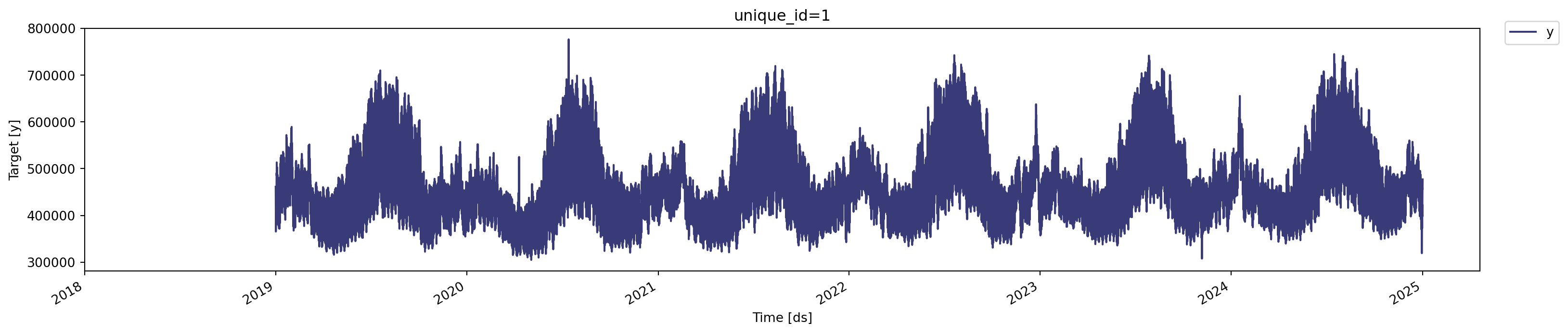

By default, the plot series uses the matplotlib library as the visualization engine. You can modify it to plotly using the engine argument:

StatsForecast.plot(ts, engine = "plotly").update_layout(height=300)

Subsetting the series

As we want to use later two full yearly cycles to train the models, we will subset the series to the last 25 months (leaving at least a month for testing). Let’s start by defining the end time of the series as the last full day (e.g., that has at least 24 hours) by finding the most recent timestamp floor and subtracting 1 hour.

end = ts["ds"].max().floor(freq = "d") - datetime.timedelta(hours = 1)

end = datetime.datetime(2024, 12, 1, 0, 0) - datetime.timedelta(hours = 1)
print(end)

2024-11-30 23:00:00

Next, let’s subtract from the end value 25 months:

start = end - datetime.timedelta(hours = 24 * 30 * 25)
print(start)

2022-11-11 23:00:00

Now, we can use the start and end values to subset the series:

df = ts[(ts["ds"] <= end) & (ts["ds"] >= start)]

df.tail()

	ds	y	unique_id
51859	2024-11-30 19:00:00	460592	1
51860	2024-11-30 20:00:00	456492	1
51861	2024-11-30 21:00:00	455024	1
51862	2024-11-30 22:00:00	462062	1
51863	2024-11-30 23:00:00	476419	1

Reploting the subset series:

StatsForecast.plot(df, engine = "plotly").update_layout(height=300)

df2 = df.copy()

df2 = df2[["ds", "y"]]
df2 = df2.rename(columns = {"ds": "period"})
df2.head()

	period	y
33863	2022-11-11 23:00:00	456403
33864	2022-11-12 00:00:00	458842
33865	2022-11-12 01:00:00	455111
33866	2022-11-12 02:00:00	448035
33867	2022-11-12 03:00:00	438165

Saving the Data Back to CSV

last but not least, let’s save the series:

df.to_csv("data/data.csv", index = False)
df2.to_csv("data/data2.csv", index = False)
ts.to_csv("data/ts_data.csv", index = False)