Visualization covid19italy with Choropleth Maps
Source:vignettes/geospatial_visualization.Rmd
geospatial_visualization.RmdThe goal of this vignette is to demonstrate methods for creating choropleth maps for the covid19 cases in Italy by province and region. We will use the rnaturalearth package to extract the geometry spital data of Italy, and mapview, ggplot2 packages to create choropleth maps of Italy province and regions.
Getting the geometry spital data
The ne_state function from the rnaturalearth package returns the geometry spital data of Italy’s province. We will set the return class to sf (Simple Features) object:
library(covid19italy)
library(rnaturalearth)
library(dplyr)

italy_map <- ne_states(country = "Italy", returnclass = "sf")

str(italy_map)
#> Classes 'sf' and 'data.frame':   110 obs. of  84 variables:
#>  $ featurecla: chr  "Admin-1 scale rank" "Admin-1 scale rank" "Admin-1 scale rank" "Admin-1 scale rank" ...
#>  $ scalerank : int  3 3 3 3 3 3 3 3 3 3 ...
#>  $ adm1_code : chr  "ITA-5442" "ITA-5437" "ITA-5451" "ITA-5452" ...
#>  $ diss_me   : int  5442 5437 5451 5452 5444 5459 5369 5441 5434 5366 ...
#>  $ iso_3166_2: chr  "IT-AO" "IT-VB" "IT-VA" "IT-CO" ...
#>  $ wikipedia : chr  NA NA NA NA ...
#>  $ iso_a2    : chr  "IT" "IT" "IT" "IT" ...
#>  $ adm0_sr   : int  1 1 1 1 1 1 1 1 1 1 ...
#>  $ name      : chr  "Aoste" "Verbano-Cusio-Ossola" "Varese" "Como" ...
#>  $ name_alt  : chr  "Aosta|Aosta Valley|Val d'Aoste|Vallée d'Aoste" "Piemont|Piémont|Piemonte|Piedmont" "Lombardy|Lombardei|Lombardie" "Lombardy|Lombardei|Lombardie" ...
#>  $ name_local: chr  NA NA NA NA ...
#>  $ type      : chr  "Province" "Province" "Province" "Province" ...
#>  $ type_en   : chr  "Province" "Province" "Province" "Province" ...
#>  $ code_local: chr  "11" "28" "21" "22" ...
#>  $ code_hasc : chr  "IT.AO" "IT.VB" "IT.VA" "IT.CO" ...
#>  $ note      : chr  "ITC" "ITC" "ITC" "ITC" ...
#>  $ hasc_maybe: chr  NA NA NA NA ...
#>  $ region    : chr  "Valle d'Aosta" "Piemonte" "Lombardia" "Lombardia" ...
#>  $ region_cod: chr  "IT-23" "IT-21" "IT-25" "IT-25" ...
#>  $ provnum_ne: int  12 13 17 17 17 19 8 13 13 21 ...
#>  $ gadm_level: int  1 1 1 1 1 1 1 1 1 1 ...
#>  $ check_me  : int  20 20 20 20 20 20 20 20 20 20 ...
#>  $ datarank  : int  3 3 3 3 3 3 3 3 3 3 ...
#>  $ abbrev    : chr  NA NA NA NA ...
#>  $ postal    : chr  "AO" "VB" "VA" "CO" ...
#>  $ area_sqkm : int  0 0 0 0 0 0 0 0 0 0 ...
#>  $ sameascity: int  NA NA NA NA NA NA NA NA NA NA ...
#>  $ labelrank : int  3 3 3 3 3 3 3 3 3 3 ...
#>  $ name_len  : int  5 20 6 4 7 5 7 5 5 6 ...
#>  $ mapcolor9 : int  8 8 8 8 8 8 8 8 8 8 ...
#>  $ mapcolor13: int  7 7 7 7 7 7 7 7 7 7 ...
#>  $ fips      : chr  "IT19" "IT12" "IT09" "IT09" ...
#>  $ fips_alt  : chr  NA NA NA NA ...
#>  $ woe_id    : int  12591856 15022642 12591884 12591808 12591881 12591814 12591858 12591824 12591807 15022641 ...
#>  $ woe_label : chr  NA NA NA NA ...
#>  $ woe_name  : chr  "Aosta" "Verbano-Cusio-Ossola" "Varese" "Como" ...
#>  $ latitude  : num  45.7 46.1 45.8 45.9 46.2 ...
#>  $ longitude : num  7.35 8.34 8.76 9.16 9.81 ...
#>  $ sov_a3    : chr  "ITA" "ITA" "ITA" "ITA" ...
#>  $ adm0_a3   : chr  "ITA" "ITA" "ITA" "ITA" ...
#>  $ adm0_label: int  2 2 2 2 2 2 2 2 2 2 ...
#>  $ admin     : chr  "Italy" "Italy" "Italy" "Italy" ...
#>  $ geonunit  : chr  "Italy" "Italy" "Italy" "Italy" ...
#>  $ gu_a3     : chr  "ITA" "ITA" "ITA" "ITA" ...
#>  $ gn_id     : int  3182996 3164567 3164697 3178227 3166396 3181912 3175531 3177699 3165523 6457404 ...
#>  $ gn_name   : chr  "Provincia di Aosta" "Provincia Verbano-Cusio-Ossola" "Provincia di Varese" "Provincia di Como" ...
#>  $ gns_id    : int  -110503 -123139 -131905 -116054 -129920 -111759 -119238 0 -130939 0 ...
#>  $ gns_name  : chr  "Valle d'Aosta, Provincia di" "Novara, Provincia di" "Varese" "Como" ...
#>  $ gn_level  : int  2 2 2 2 2 2 2 2 2 2 ...
#>  $ gn_region : chr  NA NA NA NA ...
#>  $ gn_a1_code: chr  "IT.AO" "IT.VB" "IT.VA" "IT.CO" ...
#>  $ region_sub: chr  NA NA NA NA ...
#>  $ sub_code  : chr  NA NA NA NA ...
#>  $ gns_level : int  2 2 2 2 2 2 2 -1 2 -1 ...
#>  $ gns_lang  : chr  NA NA NA NA ...
#>  $ gns_adm1  : chr  NA NA NA NA ...
#>  $ gns_region: chr  "IT19" "IT12" "IT09" "IT09" ...
#>  $ min_label : num  9 9 9 9 9 9 9 9 9 9 ...
#>  $ max_label : num  11 11 11 11 11 11 11 11 11 11 ...
#>  $ min_zoom  : num  9 9 9 9 9 9 9 9 9 9 ...
#>  $ wikidataid: chr  "Q3367" "Q16312" "Q16299" "Q16161" ...
#>  $ name_ar   : chr  NA NA NA NA ...
#>  $ name_bn   : chr  NA NA NA NA ...
#>  $ name_de   : chr  "Aosta" "Provinz Verbano-Cusio-Ossola" "Provinz Varese" "Provinz Como" ...
#>  $ name_en   : chr  "Aosta" "province of Verbano-Cusio-Ossola" "Province of Varese" "Province of Como" ...
#>  $ name_es   : chr  "Aosta" "Verbano-Cusio-Ossola" "Varese" "Como" ...
#>  $ name_fr   : chr  "Aoste" "province du Verbano-Cusio-Ossola" "Province de Varèse" "province de Côme" ...
#>  $ name_el   : chr  NA NA NA NA ...
#>  $ name_hi   : chr  NA NA NA NA ...
#>  $ name_hu   : chr  "Aosta" "Verbano-Cusio-Ossola megye" "Varese megye" "Como megye" ...
#>  $ name_id   : chr  "Aosta" "Provinsi Verbano-Cusio-Ossola" "Provinsi Varese" "Provinsi Como" ...
#>  $ name_it   : chr  "Aosta" "provincia del Verbano-Cusio-Ossola" "provincia di Varese" "provincia di Como" ...
#>  $ name_ja   : chr  NA NA NA NA ...
#>  $ name_ko   : chr  NA NA NA NA ...
#>  $ name_nl   : chr  "Aosta" "Verbano-Cusio-Ossola" "Varese" "Como" ...
#>  $ name_pl   : chr  "Aosta" "Prowincja Cusio Ossola" "Prowincja Varese" "Prowincja Como" ...
#>  $ name_pt   : chr  "Aosta" "Verbano Cusio Ossola" "Varese" "Como" ...
#>  $ name_ru   : chr  NA NA NA NA ...
#>  $ name_sv   : chr  "Aosta" "Verbano Cusio Ossola" "Varese" "Como" ...
#>  $ name_tr   : chr  "Aosta" "Verbano-Cusio-Ossola ili" "Varese ili" "Como ili" ...
#>  $ name_vi   : chr  "Aosta" "Verbano-Cusio-Ossola" "Varese" "Como" ...
#>  $ name_zh   : chr  NA NA NA NA ...
#>  $ ne_id     : chr  "1159310915" "1159316907" "1159316941" "1159316943" ...
#>  $ geometry  :sfc_MULTIPOLYGON of length 110; first list element: List of 1
#>   ..$ :List of 1
#>   .. ..$ : num [1:149, 1:2] 7.02 7.07 7.09 7.12 7.15 ...
#>   ..- attr(*, "class")= chr  "XY" "MULTIPOLYGON" "sfg"
#>  - attr(*, "sf_column")= chr "geometry"
#>  - attr(*, "agr")= Factor w/ 3 levels "constant","aggregate",..: NA NA NA NA NA NA NA NA NA NA ...
#>   ..- attr(*, "names")= chr  "featurecla" "scalerank" "adm1_code" "diss_me" ...
The function returns many features, such as a different naming convention. However, for the purpose of this vignette, we will only need the following columns:
-
name- the province name -
region- the region name -
geometry- the geometry spital data of the provinces
italy_map <- italy_map %>%
  select(province = name, region, geometry)

head(italy_map)
#> Simple feature collection with 6 features and 2 fields
#> geometry type:  MULTIPOLYGON
#> dimension:      XY
#> bbox:           xmin: 6.781994 ymin: 45.46629 xmax: 12.46963 ymax: 47.08521
#> CRS:            +proj=longlat +datum=WGS84 +no_defs +ellps=WGS84 +towgs84=0,0,0
#>                 province              region                       geometry
#> 399                Aoste       Valle d'Aosta MULTIPOLYGON (((7.022083 45...
#> 401 Verbano-Cusio-Ossola            Piemonte MULTIPOLYGON (((7.84962 45....
#> 403               Varese           Lombardia MULTIPOLYGON (((8.728974 46...
#> 404                 Como           Lombardia MULTIPOLYGON (((8.908885 45...
#> 406              Sondrio           Lombardia MULTIPOLYGON (((9.224831 46...
#> 407                Bozen Trentino-Alto Adige MULTIPOLYGON (((10.45183 46...
The italy_map object, as it is, can now use to create a choropleth map plot for the province level. To get a similar object to the regional level, we will use the dplyr package to group the data by the region column. This will automatically will group the geometry objects of the italy_map to the region level:
italy_map_region <- italy_map %>%
  group_by(region) %>%
  summarise(n = n())

head(italy_map_region)
#> Simple feature collection with 6 features and 2 fields
#> geometry type:  GEOMETRY
#> dimension:      XY
#> bbox:           xmin: 9.201431 ymin: 37.91901 xmax: 18.51743 ymax: 45.13849
#> CRS:            +proj=longlat +datum=WGS84 +no_defs +ellps=WGS84 +towgs84=0,0,0
#> # A tibble: 6 x 3
#>   region           n                                                    geometry
#>   <chr>        <int>                                              <GEOMETRY [°]>
#> 1 Abruzzo          4 POLYGON ((14.25716 42.44607, 14.28419 42.42829, 14.35621 4…
#> 2 Apulia           6 POLYGON ((18.09893 40.51793, 18.11997 40.50458, 18.21168 4…
#> 3 Basilicata       2 POLYGON ((16.86328 40.39092, 16.78273 40.30158, 16.7614 40…
#> 4 Calabria         5 POLYGON ((16.57349 38.46733, 16.56959 38.42951, 16.56137 3…
#> 5 Campania         5 MULTIPOLYGON (((13.94467 40.70161, 13.93483 40.70563, 13.9…
#> 6 Emilia-Roma…     9 POLYGON ((12.49074 43.96504, 12.48919 43.97311, 12.48216 4…
Note that since we had to feed some variable to the summarise function, we used the n function as a dummy variable.
Now, we have a geometric object for the provinces and regions levels, we can merge them with the corresponding datasets - italy_province and italy_region. Each dataset ha
The province_spatial and region_spatial columns on the italy_province and italy_region datasets are the default provinces and regions names as used in the rnatualearth package spatial objects, and we will use them to merge the objects:
italy_map_region <- italy_map_region %>%
  left_join(italy_region %>%
              filter(date == max(date)), # subseting for the most recent day
            by = c("region" = "region_spatial"))


italy_map_province <- italy_map %>%
  left_join(italy_province %>%
              filter(date == max(date)), # subseting for the most recent day
            by = c("province" = "province_spatial"))
Now that we have one object for the province level and one for the regional level, we can start to plot them.
Choropleth maps with the mapview package
The mapview package provides interactive visualisations of spatial data based on the Leaflet JavaScript library. In the following example we will plot the total number of covide19 cases in Italy as of 2021-07-27, using the total_cases variable:
Note: the Italy province spatial data on the rnaturalearth package is not updated with changes in the provinces of the Sardegna region that occurred in 2016. Therefore, some of the provinces in that region is missing from the plot. Alternatively, you can download Italy shapefile from the European Environment Agency website. However, the use of shapefiles is not cover on this vignette.
The col.regions argument enables to set the color pallet of the choropleth map. For example, we will use the plasma color pallet from the viridisLite package:
Similarly, we can plot the region level total number of tests conduct as of 2021-07-27:
italy_map_region %>%
  mapview(zcol = "total_tests")
Additional customization options can be found on the mapview package site
Choropleth maps with the ggplot2 package
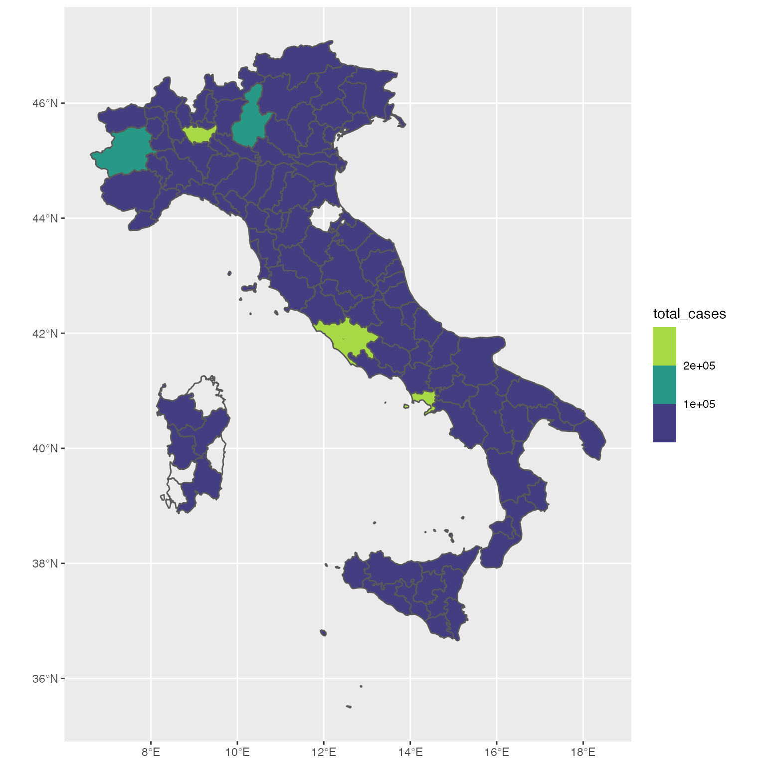
Once the geometric objects of the province and region levels are ready, it is straightforward to plot the mops with the ggplot2 package. For example, let’s plot the total number of testing again, this time with ggplot2:
library(ggplot2)
ggplot(data = italy_map_province, aes(fill = `total_cases`)) +
  geom_sf() +
  scale_fill_viridis_b()
Customizations of the plot color palette can be done with the scale_fill_viridis_b argument. For example, by default, the function uses the viridis palette from the viridis package. We can modify the palette to magma, by setting the option argument to A:
ggplot(data = italy_map_province, aes(fill = `total_cases`)) +
  geom_sf() +
    scale_fill_viridis_b(option = "A",
                       begin = 0.2,
                       end = 0.7) +
   theme_void()
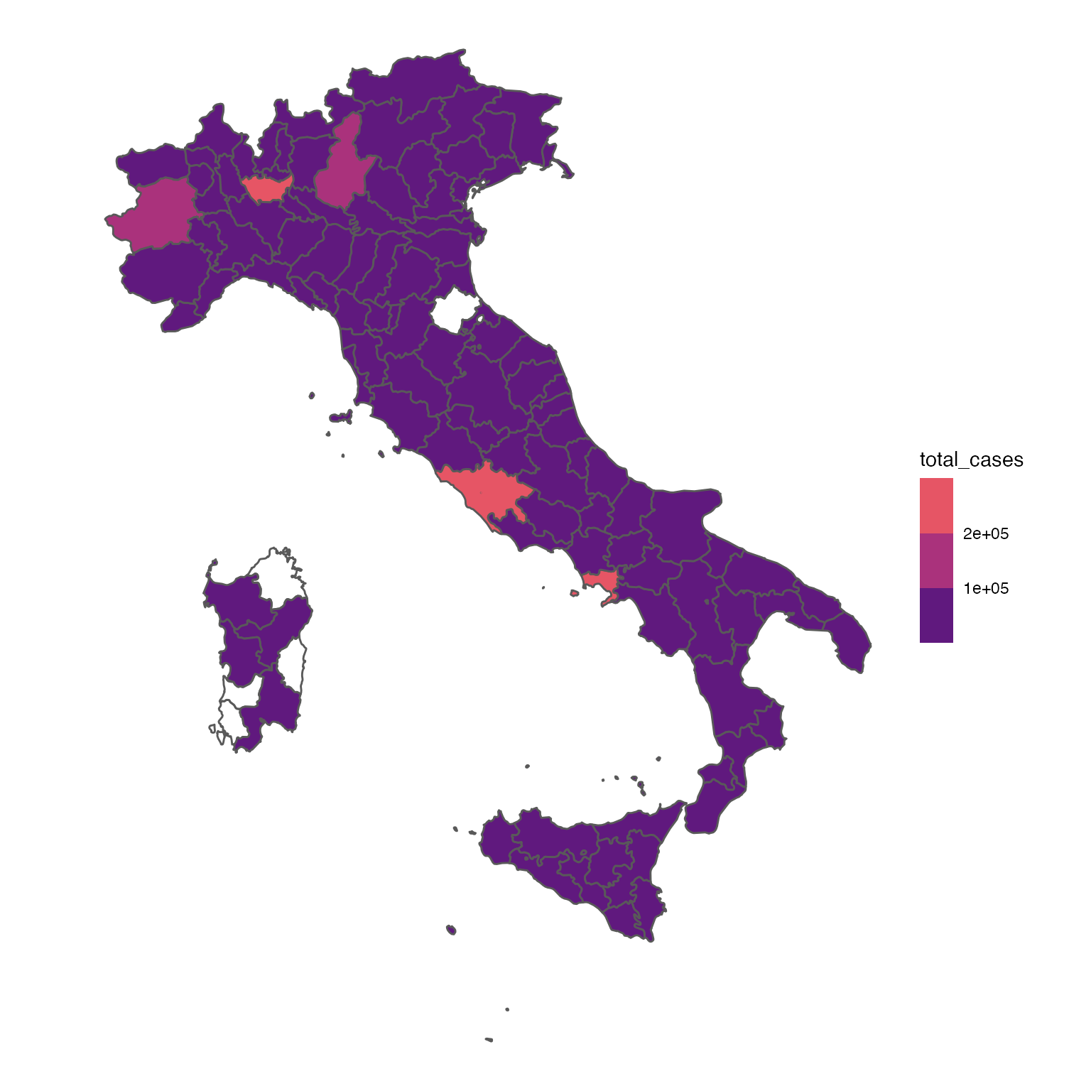
The theme_void remove the axis grids and the gray background.