The covid19sf_geo provides information about San Francisco Covid19 cases distribution by geospatial location. Also, testing locations across San Francisco available on covid19sf_test_loc dataset. The following vignette provides examples for geospatial visualization of those datasets. Both datasets are sf objects and contain geometric information (i.e., ready to plot on a map).
Note: This is a non-CRAN vignette, and the following libraries required to build the plots on this document:
The covid19sf_geo dataset
The covid19sf_geo dataset provides a snapshot of the distribution of the Covid19 cases in San Francisco by different geographic locations splits of the city. The dataset contains the following fields:
-
area_type- the geograpichal split method:-
ZCTAfor view the data by ZIP code -
Analysis Neighborhoodfor view the data by neigborhoods -
Census Tractfor view the data by census tract, and -
Citywidefor total cases in the city
-
-
id- the area ID (e.g., ZIP code, neighborhood name, etc.) -
count- total number of positive cases in the area -
rate- cases rate per 10000 residents -
deaths- total number of deaths in the area -
acs_population- total number of residents in the area -
last_updated- most recent update time of the dataset
While the first three geographical split methods contain geometry components that enable us to plot them as a map, the last is just an aggregated summary of the city’s total cases.
library(covid19sf)

data(covid19sf_geo)

class(covid19sf_geo)
#> [1] "sf"         "data.frame"

head(covid19sf_geo)
#> Simple feature collection with 6 features and 7 fields
#> Geometry type: MULTIPOLYGON
#> Dimension:     XY
#> Bounding box:  xmin: -122.4543 ymin: 37.70792 xmax: -122.357 ymax: 37.80602
#> Geodetic CRS:  WGS 84
#>               area_type                             id count      rate deaths
#> 1 Analysis Neighborhood          Bayview Hunters Point  5314 1401.4822     37
#> 2 Analysis Neighborhood                 Bernal Heights  1729  687.0108     NA
#> 3 Analysis Neighborhood            Castro/Upper Market  1211  538.1744     15
#> 4 Analysis Neighborhood                      Chinatown   561  388.5580     17
#> 5 Analysis Neighborhood                      Excelsior  3347  839.2888     27
#> 6 Analysis Neighborhood Financial District/South Beach  1309  607.7912     NA
#>   acs_population        last_updated                       geometry
#> 1          37917 2021-12-14 08:30:14 MULTIPOLYGON (((-122.3936 3...
#> 2          25167 2021-12-14 08:30:14 MULTIPOLYGON (((-122.4036 3...
#> 3          22502 2021-12-14 08:30:14 MULTIPOLYGON (((-122.4266 3...
#> 4          14438 2021-12-14 08:30:14 MULTIPOLYGON (((-122.4062 3...
#> 5          39879 2021-12-14 08:30:14 MULTIPOLYGON (((-122.425 37...
#> 6          21537 2021-12-14 08:30:14 MULTIPOLYGON (((-122.3875 3...
Plotting cases with mapview
The most intuitive method for plotting sf objects is with the mapview package, which is a wrapper for the leaflet JavaScript package. The main advantage of the mapview package that it is both interactive and smoothly works with sf objects. The following example demonstrated the use case of the mapview function to plot the confirmed cases in San Francisco with the plot function to plot cases distribution by ZIP code:
You can use at and col.regions arguments to define color buckets and color range, respectively:
Plotting vaccine data with tmap
The tmap package provides functions and tools for creating thematic maps. The package supports sf objects and follow the ggplot2 framework. In the example below we will plot the COVID-19 vaccine data by geographic using the covid19sf_vaccine_geo dataset:
data(covid19sf_vaccine_geo)

head(covid19sf_vaccine_geo)
#> Simple feature collection with 6 features and 8 fields
#> Geometry type: MULTIPOLYGON
#> Dimension:     XY
#> Bounding box:  xmin: -122.4773 ymin: 37.73155 xmax: -122.3843 ymax: 37.80602
#> Geodetic CRS:  WGS 84
#>                               id             area_type count_vaccinated_by_dph
#> 1                 Bernal Heights Analysis Neighborhood                    5106
#> 2 Financial District/South Beach Analysis Neighborhood                    1841
#> 3                      Glen Park Analysis Neighborhood                     573
#> 4                 Haight Ashbury Analysis Neighborhood                     823
#> 5                   Hayes Valley Analysis Neighborhood                    2401
#> 6                   Inner Sunset Analysis Neighborhood                    1220
#>   count_vaccinated count_series_completed acs_population
#> 1            21109                  19781          25167
#> 2            22782                  20215          21537
#> 3             7257                   6804           8651
#> 4            14360                  13279          19275
#> 5            16351                  14930          19711
#> 6            23414                  21829          29539
#>   percent_pop_series_completed        last_updated
#> 1                    0.7859896 2021-12-15 04:45:07
#> 2                    0.9386173 2021-12-15 04:45:09
#> 3                    0.7864987 2021-12-15 04:45:09
#> 4                    0.6889235 2021-12-15 04:45:09
#> 5                    0.7574451 2021-12-15 04:45:09
#> 6                    0.7389891 2021-12-15 04:45:09
#>                         geometry
#> 1 MULTIPOLYGON (((-122.4036 3...
#> 2 MULTIPOLYGON (((-122.3875 3...
#> 3 MULTIPOLYGON (((-122.4474 3...
#> 4 MULTIPOLYGON (((-122.432 37...
#> 5 MULTIPOLYGON (((-122.4208 3...
#> 6 MULTIPOLYGON (((-122.4529 3...
Additional setting: Following changes in the default options of the sf package from version 1.0-1 by default option is to use s2 spherical geometry as default when coordinates are ellipsoidal. That cause some issues with the tmap package, therefore we will set this functionality as FALSE:
sf_use_s2(FALSE)
#> Spherical geometry (s2) switched off
We will use the percent_pop_series_completed variable to plot the percentage of population that finished their vaccination process. Let’s first filter the data and transform the percent_pop_series_completed from decimal to percentage:
df <- covid19sf_vaccine_geo %>% filter(area_type == "Analysis Neighborhood") %>%
  dplyr::mutate(perc_complated = percent_pop_series_completed * 100)
Now we can plot the new object:
tm_shape(df) +
  tm_polygons("perc_complated",
              title = "% Group")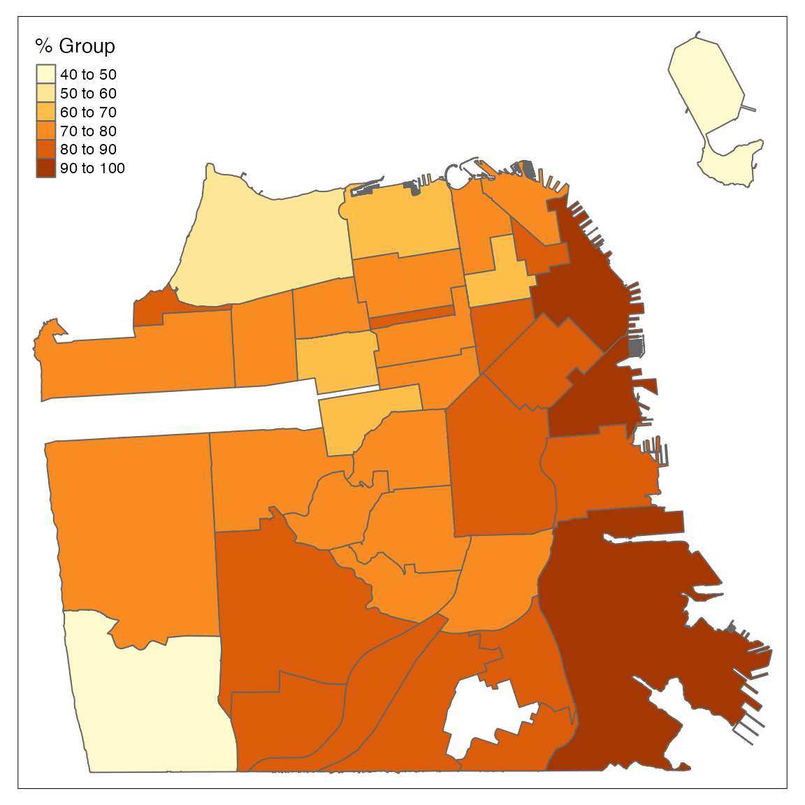
By default, the tm_polygons function bucket the numeric variable, in this case percentage of vaccinated population, into buckets. You can control the number of buckets using the n argument. Let’s now start to customize the plot and modify to color palette:
tm_shape(df) +
  tm_polygons("perc_complated",
              title = "% Group",
              palette = "RdYlBu")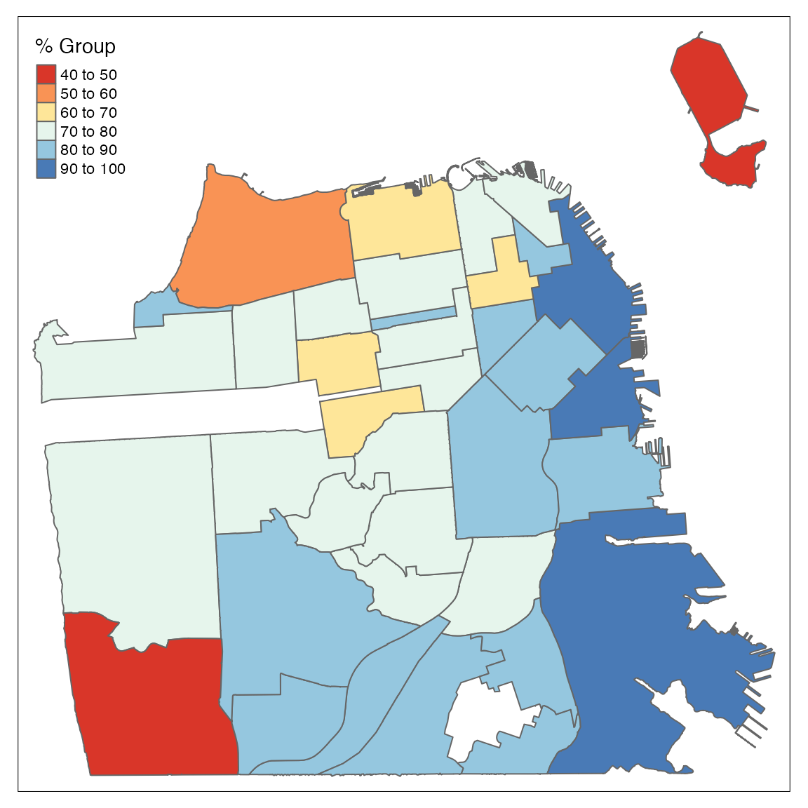
We can customize the plot background with the tm_style function by using the style argument:
tm_shape(df) +
  tm_polygons("perc_complated",
              title = "% Group",
              palette = "RdYlBu") +
  tm_style(style = "cobalt")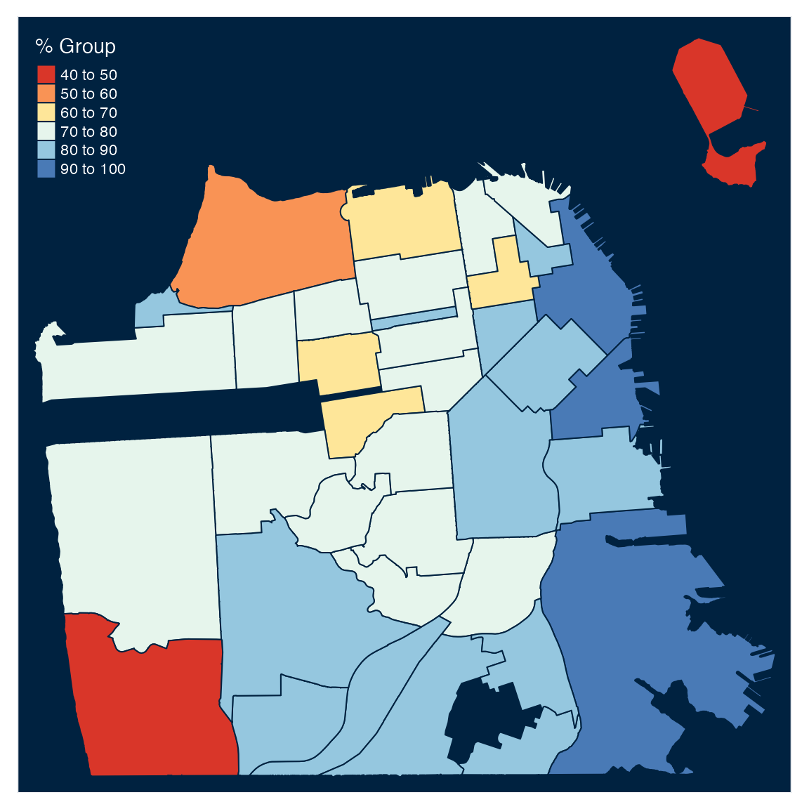
Last but not least, let’s add title and labels for the geographic locations with the tm_text and tm_layout functions:
tm_shape(df) +
  tm_polygons("perc_complated",
              title = "% Group",
              palette = "RdYlBu") +
  tm_style("cobalt") +
  tm_text("id", size = 0.5) +
  tm_layout(
    legend.position=c("right", "bottom"),
    legend.outside = FALSE,
    legend.width = 1,
    legend.title.size = 1.2,
    legend.text.size = 1,
    # legend.outside.size = 0.9,
    title= paste("COVID-19 Vaccines Given",
                 "to San Franciscans by Geography",
                 sep = " "),
    title.position = c("left", "top") ,
inner.margins = c(0.01, .01, .12, .25)) 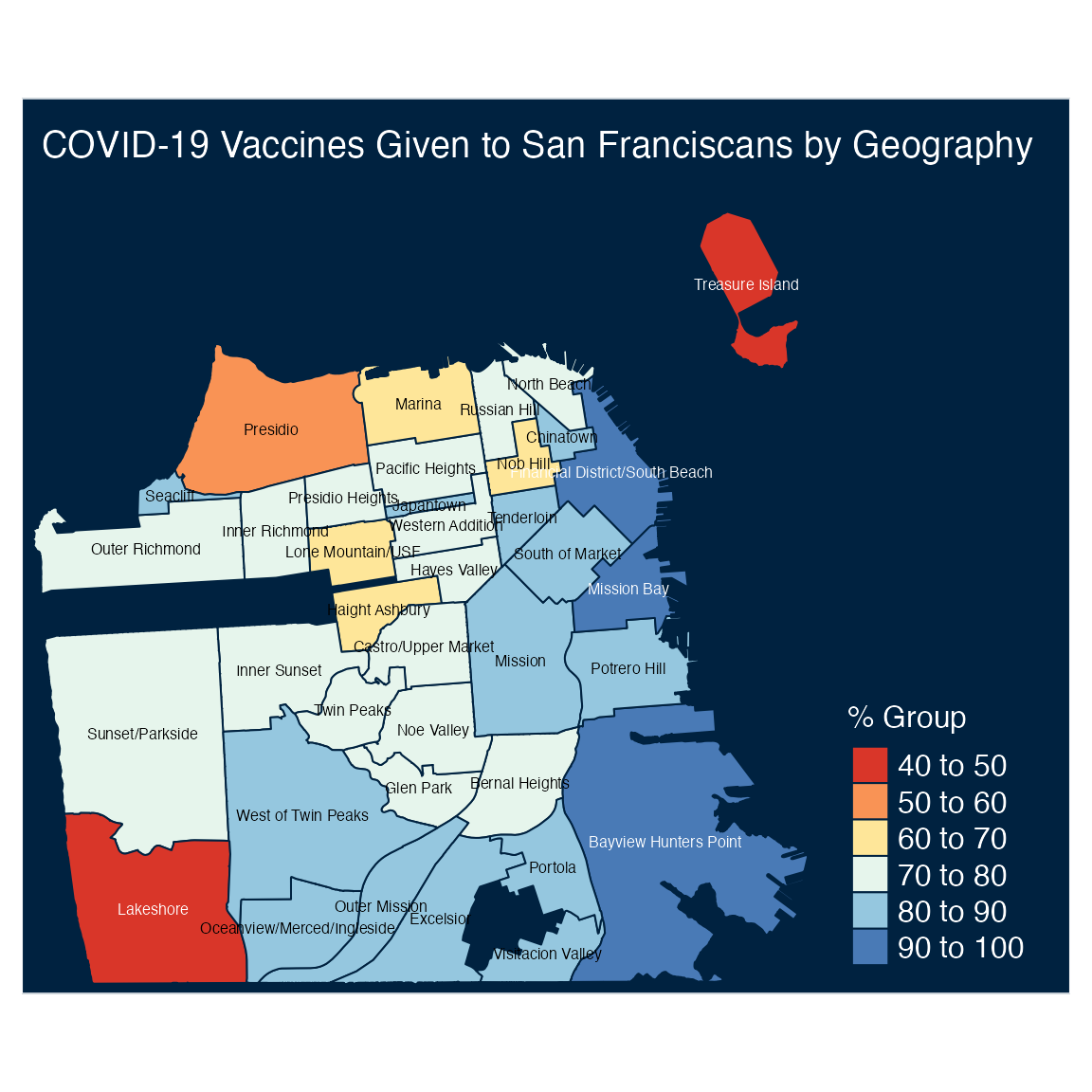
Plotting cases with base plot
The sf package provides a plot method for sf objects (see ?sf:::plot.sf for more information). Similarly to the previews examples above, we will replot the confirmed cases by ZIP code with the plot function:
zip <- covid19sf_geo %>%
  dplyr::filter(area_type == "ZCTA") %>%
  dplyr::select(count, geometry) %>%
  plot(main = "Covid19 Cases by ZIP Code")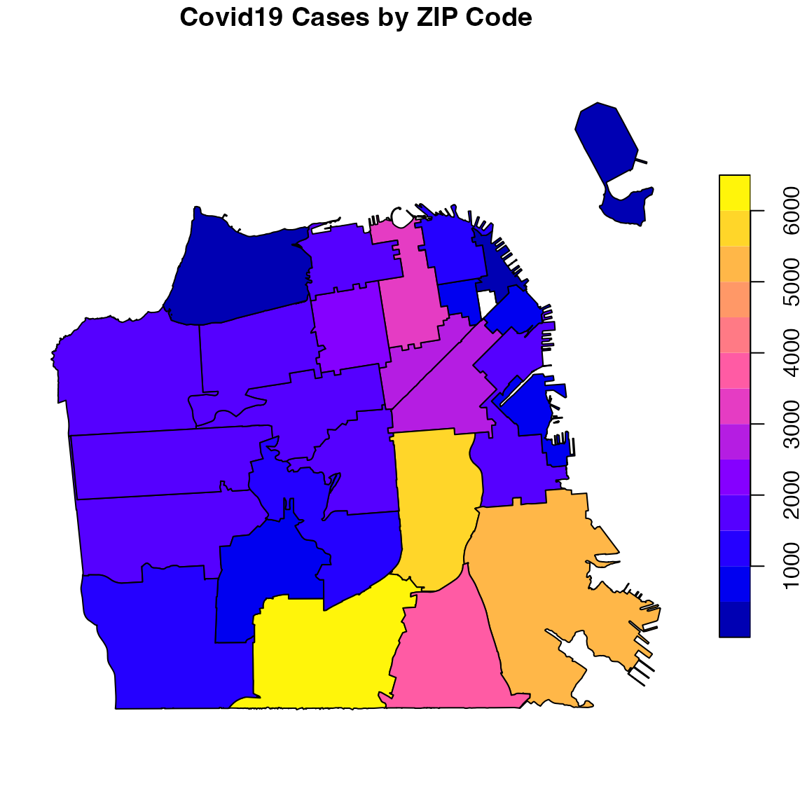
You can define the color palette with the pal argument and set the level of breaks of the color scale by setting the breaks argument to quantile and the number of breaks with the nbreaks argument (which should be aligned with the number of colors on the color palette):
library(RColorBrewer)
pal <- brewer.pal(9, "OrRd")

covid19sf_geo %>%
  filter(area_type == "ZCTA") %>%
  select(count, geometry) %>%
  plot(main = "Covid19 Cases by ZIP Code",
       breaks = "quantile", nbreaks = 9,
       pal = pal)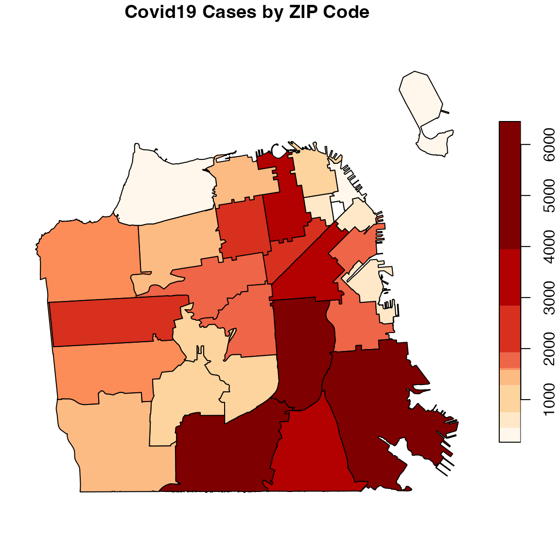
Plotting cases with ggplot2
Plotting sf object can be done with the ggplot2 package natively by using the geom_sf function for plotting sf objects:
library(ggplot2)

covid19sf_geo %>%
  filter(area_type == "ZCTA") %>%
  ggplot() +
  geom_sf(aes(fill=count)) +
  ggtitle("Covid19 Cases by ZIP Code")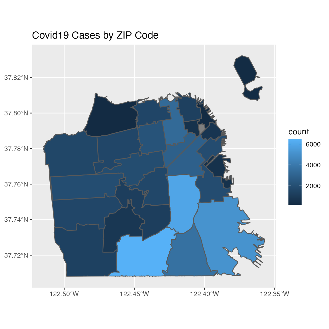
You can customize the polygon color scale by using the scale_viridis function that enables you to select different viridis color palettes. In addition, the geom_sf_label enables you to add labels for each polygon. In the next example, we will replot the count of cases by ZIP code, this time using scale_fill_viridis_b color palette and setting the id variable as the polygon title using the geom_sf_label:
covid19sf_geo %>%
  filter(area_type == "ZCTA") %>%
  ggplot() +
  geom_sf(aes(fill=count)) +
  scale_fill_viridis_b() +
  geom_sf_label(aes(label = id)) +
  ggtitle("Covid19 Cases by ZIP Code")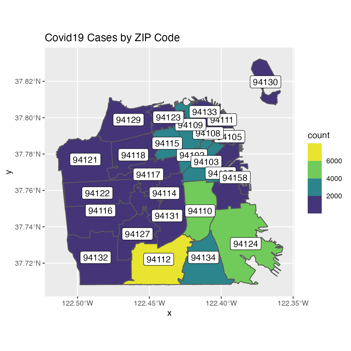
Additional customization of the viridis color palettes can be done by the option argument, where the begin, and end arguments control the color hue:
covid19sf_geo %>%
  filter(area_type == "ZCTA") %>%
  ggplot() +
  geom_sf(aes(fill=count)) +
    scale_fill_viridis_b(option = "A",
                       begin = 0.2,
                       end = 0.7) +
   theme_void() +
  ggtitle("Covid19 Cases by ZIP Code")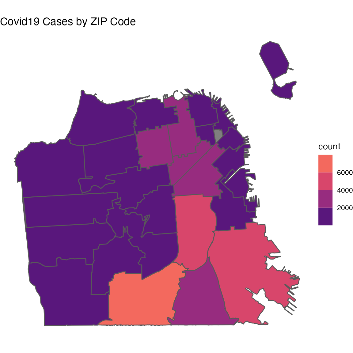
The covid19sf_test_loc dataset
The covid19sf_test_loc datasets provides general metadata about the Covid19 testing locations in San Francisco:
data(covid19sf_test_loc)

head(covid19sf_test_loc)
#> Simple feature collection with 6 features and 16 fields
#> Geometry type: POINT
#> Dimension:     XY
#> Bounding box:  xmin: -122.4486 ymin: 37.7187 xmax: -122.3849 ymax: 37.78699
#> Geodetic CRS:  WGS 84
#>   id                                             medical_home
#> 1  6                                                     UCSF
#> 2  1                                            Carbon Health
#> 3 11                               Northeast Medical Services
#> 4 43 SF Department of Public Health in partnership with Color
#> 5 25 SF Department of Public Health in partnership with Color
#> 6 38                                                     <NA>
#>                              name                 address phone_number
#> 1           Laurel Heights Campus      3333 California St   4158857478
#> 2   Carbon Health - Castro Clinic          1998 Market St   4157926040
#> 3            San Bruno Ave Clinic      2574 San Bruno Ave   4153919686
#> 4                  Alice Griffith 2600 Arelious Walker Dr          311
#> 5           GLIDE Memorial Church        330 Ellis Street          311
#> 6 Test the People by renegade.bio            2730 21st St   5103273540
#>   phone_number_formatted                                  testing_hours
#> 1         (415) 885-7478                                    9am-5pm M-F
#> 2         (415) 792-6040                                        9am-7pm
#> 3         (415) 391-9686                                 8:30am-5pm M-F
#> 4             Dial 3-1-1           Saturday, 11/20 only from 10am - 3pm
#> 5             Dial 3-1-1                Tuesdays & Wednesdays, 10am-4pm
#> 6         (510) 327-3540 M, W, and F from 10 AM to 3PM, except holidays
#>   popup_or_permanent location_type
#> 1             Pop-Up       Private
#> 2          Permanent       Private
#> 3          Permanent       Private
#> 4             Pop-Up        Public
#> 5             Pop-Up        Public
#> 6             Pop-Up       Private
#>                                                         eligibility
#> 1                                              Must be UCSF patient
#> 2                                     Must be Carbon Health patient
#> 3 Must be NEMS patient. May register as a new NEMS patient for free
#> 4                                  Everyone. No insurance required.
#> 5                                  Everyone. No insurance required.
#> 6                                  Everyone. No insurance required.
#>                                 cta_text
#> 1            Physician referral required
#> 2                  Sign up with provider
#> 3                  Sign up with provider
#> 4                                Drop in
#> 5                               Drop in.
#> 6 Drop in or call ahead for appointments
#>                                                                                                                                                                                                                               cta_link
#> 1                                                                                                                                                                                                                     tel://4158857478
#> 2 https://patient.carbonhealth.com/#/schedule?practiceId=5bdaef44-8ff0-439f-99d7-3285afcc6911&vstId=0f02af4e-1d1c-4a4b-a0f2-e67fca98dd77&vstrId=f743d1d1-d2a1-4fce-a5f9-2e29339b2406&specialtyIds=652c64cc-9fcb-442f-b71e-266390ef2f63
#> 3                                                                                                                                                                                                        https://www.nems.org/covid19/
#> 4                                                                                                                                                                                                           https://sf.gov/GetTestedSF
#> 5                                                                                                                                                                                                           https://sf.gov/GetTestedSF
#> 6                                                                                                                                                                                                       https://www.testthepeople.org/
#>   sample_collection_method                       lab   latitude    longitude
#> 1                     <NA>                      UCSF       <NA>         <NA>
#> 2                     <NA> Rapid test (Abbot ID NOW)       <NA>         <NA>
#> 3                     <NA>                      <NA>       <NA>         <NA>
#> 4                     <NA>                      <NA> 37.7187018 -122.3849448
#> 5                     <NA>                      <NA> 37.7852341  -122.413658
#> 6                     <NA>                      <NA>  37.757629 -122.4094428
#>                     geometry
#> 1 POINT (-122.4486 37.78699)
#> 2 POINT (-122.4259 37.77001)
#> 3  POINT (-122.4042 37.7291)
#> 4  POINT (-122.3849 37.7187)
#> 5 POINT (-122.4137 37.78523)
#> 6 POINT (-122.4094 37.75763)
Plotting the testing locations on map is fairly similar to one of the covid19sf_geo as both are sf objects. The main distinction between the two, is that the covid19sf_test_loc provides the geometry location (e.g., latitude and longitude) as opposed to a polygon. Let’s plot the locations with the mapview package setting the location color by the type (private or public):
Combine cases dist. and testing points
The sync function from the leafsync package enables to combine multiple maps plots. In the following example, we will put side by side the cases split by ZIP code and the testing point in the city map:
m1 <- covid19sf_geo %>%
  filter(area_type == "ZCTA") %>%
  mapview(zcol = "count",
          at = c(0,  200, 400, 800, 1200, 1600, 2000),
          col.regions = (c('#fef0d9','#b30000')))
m2 <- covid19sf_test_loc %>% mapview(zcol = "location_type")
sync(m1, m2)