Geospatial Visualization
Source:vignettes/geospatial_visualization.Rmd
geospatial_visualization.RmdThe coronavirus and covid19_vaccine datasets provide country-level information on the COVID-19 cases and vaccination progress, respectively. A common method to communicate and visualize country-level data is with the use of choropleth maps. This vignette focuses on approaches for plotting COVID-19 cases with choropleth maps using the following packages:
rnaturalearth - Provides geo-spatial metadata from the Natural Earth dataset. More details available here
sf - A package that provides simple features access for R
mapview - A wrapper for the leaflet library
tmap - A package for creating a thematic maps
ggplot2 - Is a system for declaratively creating graphics
viridis - A package that provide a series of color maps
Note: This vignette is not available on the CRAN version (due to size limitations). Therefore, as the packages above are not on the dependencies list of the coronavirus package, you may need to install them before.
Additional setting: following changes in the default options of the sf package from version 1.0-1 by default option is to use s2 spherical geometry as default when coordinates are ellipsoidal. That causes some issues with the tmap package, therefore we will set this functionality as FALSE:
sf_use_s2(FALSE)
#> Spherical geometry (s2) switched off
More details are available on this issue and follow-up issue.
Data prep
Let’s get started by loading the data:
library(coronavirus)

data("covid19_vaccine")

head(covid19_vaccine)
#>         date country_region continent_name continent_code combined_key
#> 1 2020-12-29        Austria         Europe             EU      Austria
#> 2 2020-12-29        Bahrain           Asia             AS      Bahrain
#> 3 2020-12-29        Belarus         Europe             EU      Belarus
#> 4 2020-12-29        Belgium         Europe             EU      Belgium
#> 5 2020-12-29         Canada  North America             NA       Canada
#> 6 2020-12-29          Chile  South America             SA        Chile
#>   doses_admin people_at_least_one_dose population uid iso2 iso3 code3 fips
#> 1        2123                     2123    9006400  40   AT  AUT    40 <NA>
#> 2       55014                    55014    1701583  48   BH  BHR    48 <NA>
#> 3           0                        0    9449321 112   BY  BLR   112 <NA>
#> 4         340                      340   11589616  56   BE  BEL    56 <NA>
#> 5       59079                    59078   37855702 124   CA  CAN   124 <NA>
#> 6          NA                       NA   19116209 152   CL  CHL   152 <NA>
#>        lat       long
#> 1  47.5162  14.550100
#> 2  26.0275  50.550000
#> 3  53.7098  27.953400
#> 4  50.8333   4.469936
#> 5  60.0000 -95.000000
#> 6 -35.6751 -71.543000
We will use the ne_countries function from the rnaturalearth package to pull the country geometric data:
library(dplyr)

map <- ne_countries(returnclass = "sf") %>%
  dplyr::select(name, iso2 = iso_a2, iso3 = iso_a3, geometry)

head(map)
#> Simple feature collection with 6 features and 3 fields
#> Geometry type: MULTIPOLYGON
#> Dimension:     XY
#> Bounding box:  xmin: -73.41544 ymin: -55.25 xmax: 75.15803 ymax: 42.68825
#> CRS:           +proj=longlat +datum=WGS84 +no_defs +ellps=WGS84 +towgs84=0,0,0
#>                   name iso2 iso3                       geometry
#> 0          Afghanistan   AF  AFG MULTIPOLYGON (((61.21082 35...
#> 1               Angola   AO  AGO MULTIPOLYGON (((16.32653 -5...
#> 2              Albania   AL  ALB MULTIPOLYGON (((20.59025 41...
#> 3 United Arab Emirates   AE  ARE MULTIPOLYGON (((51.57952 24...
#> 4            Argentina   AR  ARG MULTIPOLYGON (((-65.5 -55.2...
#> 5              Armenia   AM  ARM MULTIPOLYGON (((43.58275 41...
df <- map %>% left_join(
   covid19_vaccine %>%
    filter(date == max(date)) %>%
    mutate(perc = round(100 * people_at_least_one_dose / population, 2)) %>%
    select(country_region, iso2, iso3, people_at_least_one_dose, perc, continent_name),
    by = c("iso2", "iso3")
)

class(df)
#> [1] "sf"         "data.frame"
After we merge the country data with the corresponding geometry data, it is straightforward to plot the data as sf object.
Choropleth maps with the mapview package
The mapview package, a wrapper for the leaflet library, enables to plot sf objects seamlessly. Let’s start by plotting the percentage of the population that fully vaccinated by country using the perc variable:
By default, the function uses a continuous color scale for the objects (in this case, percentage of population that is vaccinated) color. We can modify it and set color buckets by using the at argument. Also, we can define the legend title with the use of the layer.name argument:
df  %>%
  mapview::mapview(zcol = "perc",
                   at = seq(0, max(df$perc, na.rm = TRUE), 10),
                   legend = TRUE,
                   layer.name = "Fully Vaccinated %")
Some of the missing values in the plot are un-populated areas such as Antarctica or a territory counted under different states such as Greenland. We can remove those and re-plot the map:
df1 <- df %>%
  filter(!name %in% c("Greenland", "Antarctica"))

df1  %>%
  mapview::mapview(zcol = "perc",
                   at = seq(0, max(df1$perc, na.rm = TRUE), 10),
                   legend = TRUE,
                   layer.name = "Fully Vaccinated %")
Last but not least, you can customize the color palette using the col.regions argument. In the following example, we will use the plasma function from the viridis package:
Choropleth maps with the tmap package
The tmap (thematic maps) package is another useful tool for creating choropleth maps. Similarly to the mapview package, the tmap package supports sf objects. This tmap follows the ggplot2 package syntax style (e.g., using the + symbol to add to the plot additional plot). We will use the tm_shape function to define the input object with the df1 object, and add the tm_polygons function to customize the plot:
tm_shape(df1) +
  tm_polygons(col = "perc",
              n = 8,
              title = "Fully Vaccinated %",
              palette = "Blues")
The projection argument enables setting the map projections method using PROJ.4 code:
tm_shape(df1) +
  tm_polygons(col = "perc",
              n = 8,
              projection = 3857,
              title = "Fully Vaccinated %",
palette = "Blues") 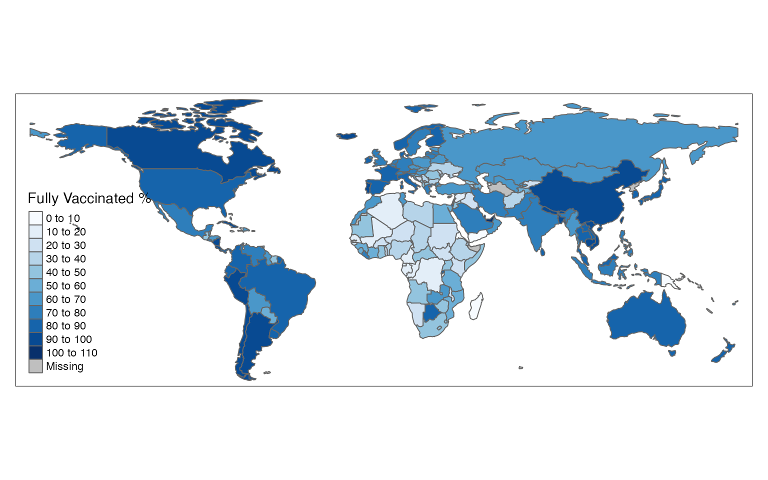
We can use the continent_name column to filter and plot the data by specific continent. For example, let’s plot the countries in South America:
df2 <- df1 %>%
  filter(continent_name == "South America")


tm_shape(df2) +
  tm_polygons(col = "perc",
              n = 5,
              title = "Perc. Group",
palette = "Blues") 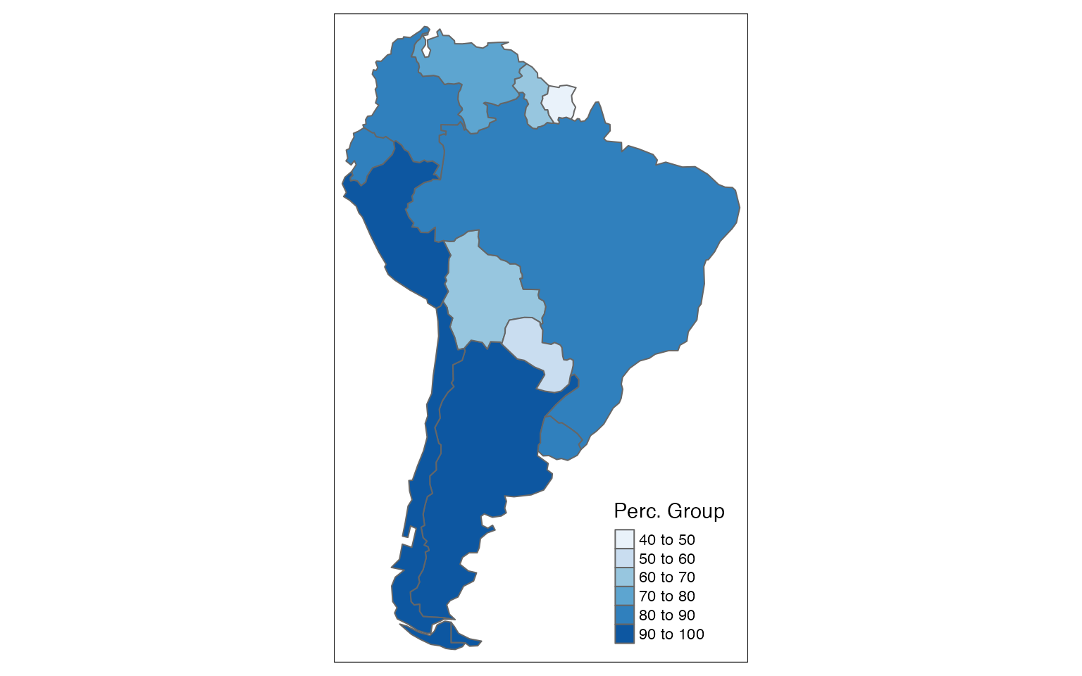
Let’s customize the plot and use the tm_stype function to set the background and the tm_layout function to add the plot title:
tm_shape(df2) +
  tm_polygons(col = "perc",
              n = 5,
              title = "Perc. Group",
              palette = "Blues") +
  tm_style("cobalt") +
  tm_text("iso3", size = 0.7) +
  tm_layout(
            title= "% of Population Fully Vaccinated",
            title.position = c('right', 'top') ,
            inner.margins = c(0.02, .02, .1, .25))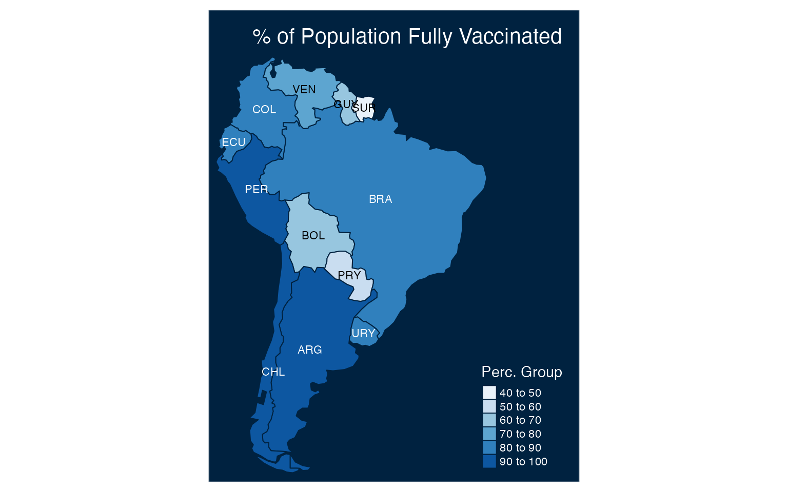
You can map the output interactive by setting the tmap_mode function to a view mode:
tmap_mode("view")

tm_shape(df2) +
  tm_polygons(col = "perc",
              n = 5,
              title = "Perc. Group",
              palette = "Blues")
Last but not least, we can add facets with the use of the tm_facets and tmap_options functions:
tmap_mode("plot")


tm_shape(df2) +
  tm_polygons(col = "perc",
              n = 5,
              title = "Perc. Group",
              palette = "Greens") +
  tmap_options(limits = c(facets.view = 13)) +
tm_facets(by = "name") 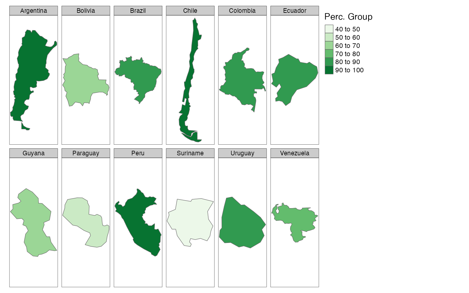
Choropleth maps with the ggplot2 package
The geom_sf function enables to read and plot sf objects with ggplot2, for example:
ggplot(data = df2, aes(fill = `perc`)) +
  geom_sf() +
  scale_fill_viridis_b()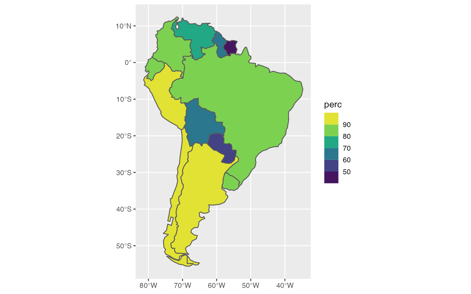
The scale_fill_viridis_b defines the color setting. By default, the y and x axes represent the earth’s coordinates. We can remove those coordinates with the theme_void function and customize the color palette with the scale_fill_viridis function:
ggplot(data = df2, aes(fill = `perc`)) +
  geom_sf(size = 0.1) +
    scale_fill_viridis(alpha = 0.9,
                       begin = 0.01,
                       discrete = FALSE,
                       end = 0.9) +
  geom_sf_label(aes(label = name)) +
  labs(fill = "Percentage",
       title = "'% of Population Fully Vaccinated",
       caption = "Source: Johns Hopkins University Center for Systems Science and Engineering") +
   theme_void()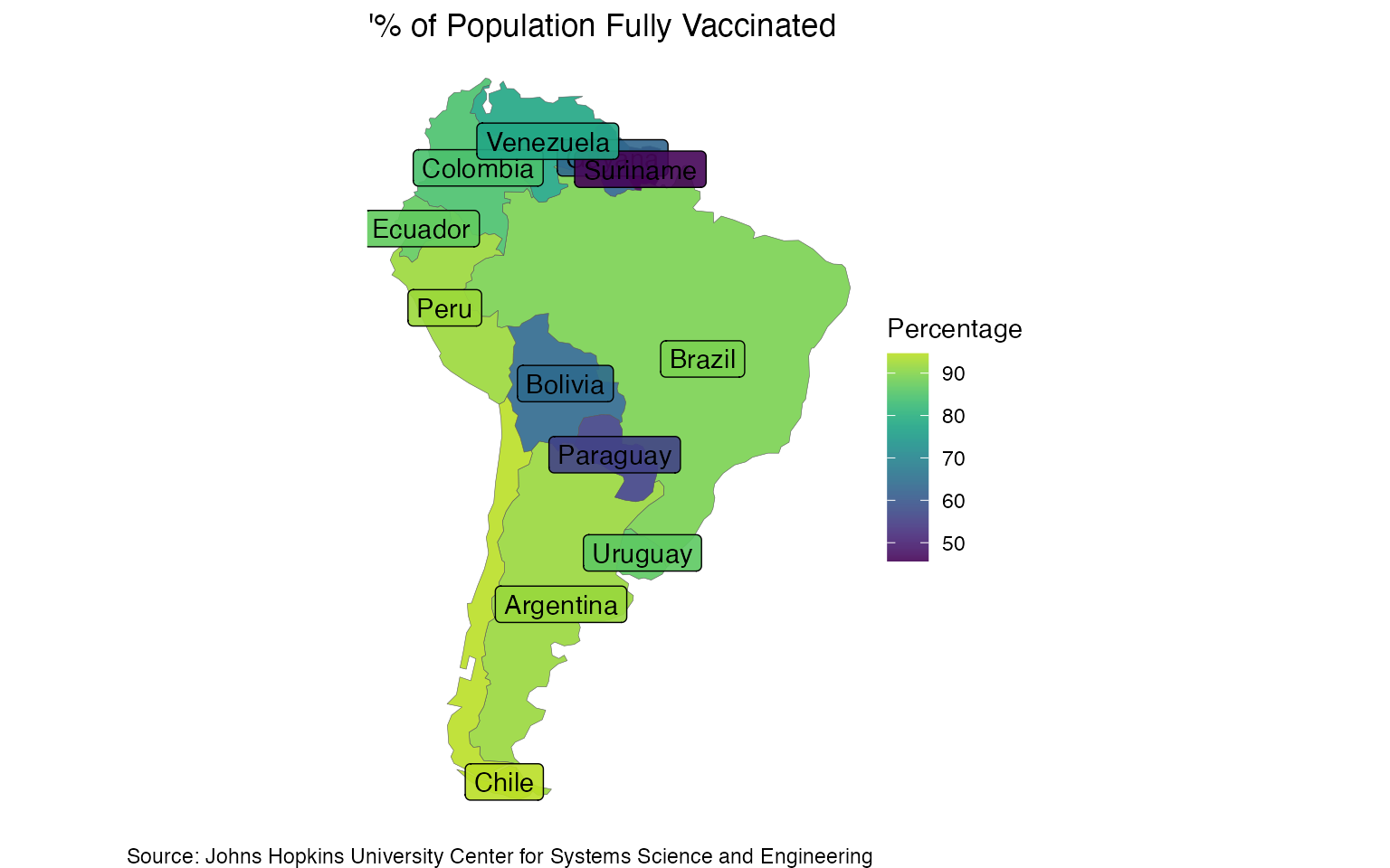
Sources:
- mapview package documentation - https://r-spatial.github.io/mapview/
- tmap package documentation - https://r-tmap.github.io/tmap/
- ggplot2 package documentation - https://ggplot2.tidyverse.org/
-
geom_sffunction - https://ggplot2.tidyverse.org/reference/ggsf.html