The 2019 Novel Coronavirus COVID-19 (2019-nCoV) Dataset • coronavirus

The coronavirus package provides a tidy format dataset of the 2019 Novel Coronavirus COVID-19 (2019-nCoV) epidemic and the vaccination efforts by country. The raw data is being pulled from the Johns Hopkins University Center for Systems Science and Engineering (JHU CCSE) Coronavirus repository.

More details available here, and a csv format of the package dataset available here

Source: Centers for Disease Control and Prevention’s Public Health Image Library

Important Notes

As this an ongoing situation, frequent changes in the data format may occur, please visit the package changelog (e.g., News) and/or see pinned issues to get updates about those changes
As of Auguest 4th JHU CCSE stopped track recovery cases, please see this issue for more details
Negative values and/or anomalies may occurred in the data for the following reasons:
- The calculation of the daily cases from the raw data which is in cumulative format is done by taking the daily difference. In some cases, some retro updates not tie to the day that they actually occurred such as removing false positive cases
- Anomalies or error in the raw data
- Please see this issue for more details

Vignettes

Additional documentation available on the followng vignettes:

Installation

Install the CRAN version:

install.packages("coronavirus")

Install the Github version (refreshed on a daily bases):

# install.packages("devtools")
devtools::install_github("RamiKrispin/coronavirus")

Datasets

The package provides the following two datasets:

coronavirus - tidy (long) format of the JHU CCSE datasets. That includes the following columns:
- date - The date of the observation, using Date class
- province - Name of province/state, for countries where data is provided split across multiple provinces/states
- country - Name of country/region
- lat - The latitude code
- long - The longitude code
- type - An indicator for the type of cases (confirmed, death, recovered)
- cases - Number of cases on given date
- uid - Country code
- province_state - Province or state if applicable
- iso2 - Officially assigned country code identifiers with two-letter
- iso3 - Officially assigned country code identifiers with three-letter
- code3 - UN country code
- fips - Federal Information Processing Standards code that uniquely identifies counties within the USA
- combined_key - Country and province (if applicable)
- population - Country or province population
- continent_name - Continent name
- continent_code - Continent code
covid19_vaccine - a tidy (long) format of the the Johns Hopkins Centers for Civic Impact global vaccination dataset by country. This dataset includes the following columns:
- country_region - Country or region name
- date - Data collection date in YYYY-MM-DD format
- doses_admin - Cumulative number of doses administered. When a vaccine requires multiple doses, each one is counted independently
- people_partially_vaccinated - Cumulative number of people who received at least one vaccine dose. When the person receives a prescribed second dose, it is not counted twice
- people_fully_vaccinated - Cumulative number of people who received all prescribed doses necessary to be considered fully vaccinated
- report_date_string - Data report date in YYYY-MM-DD format
- uid - Country code
- province_state - Province or state if applicable
- iso2 - Officially assigned country code identifiers with two-letter
- iso3 - Officially assigned country code identifiers with three-letter
- code3 - UN country code
- fips - Federal Information Processing Standards code that uniquely identifies counties within the USA
- lat - Latitude
- long - Longitude
- combined_key - Country and province (if applicable)
- population - Country or province population
- continent_name - Continent name
- continent_code - Continent code

Data refresh

While the coronavirus CRAN version is updated every month or two, the Github (Dev) version is updated on a daily bases. The update_dataset function enables to overcome this gap and keep the installed version with the most recent data available on the Github version:

library(coronavirus)
update_dataset()

Note: must restart the R session to have the updates available

Alternatively, you can pull the data using the Covid19R project data standard format with the refresh_coronavirus_jhu function:

covid19_df <- refresh_coronavirus_jhu()
head(covid19_df)
#>         date    location location_type location_code location_code_type
#> 1 2022-04-21 Afghanistan       country            AF         iso_3166_2
#> 2 2022-04-20 Afghanistan       country            AF         iso_3166_2
#> 3 2021-12-26 Afghanistan       country            AF         iso_3166_2
#> 4 2022-04-17 Afghanistan       country            AF         iso_3166_2
#> 5 2022-04-23 Afghanistan       country            AF         iso_3166_2
#> 6 2022-04-24 Afghanistan       country            AF         iso_3166_2
#>    data_type value      lat     long
#> 1 deaths_new     0 33.93911 67.70995
#> 2 deaths_new     0 33.93911 67.70995
#> 3 deaths_new     5 33.93911 67.70995
#> 4 deaths_new     2 33.93911 67.70995
#> 5 deaths_new     1 33.93911 67.70995
#> 6 deaths_new     1 33.93911 67.70995

Usage

data("coronavirus")

head(coronavirus)
#>         date province country     lat      long      type cases   uid iso2 iso3
#> 1 2020-01-22  Alberta  Canada 53.9333 -116.5765 confirmed     0 12401   CA  CAN
#> 2 2020-01-23  Alberta  Canada 53.9333 -116.5765 confirmed     0 12401   CA  CAN
#> 3 2020-01-24  Alberta  Canada 53.9333 -116.5765 confirmed     0 12401   CA  CAN
#> 4 2020-01-25  Alberta  Canada 53.9333 -116.5765 confirmed     0 12401   CA  CAN
#> 5 2020-01-26  Alberta  Canada 53.9333 -116.5765 confirmed     0 12401   CA  CAN
#> 6 2020-01-27  Alberta  Canada 53.9333 -116.5765 confirmed     0 12401   CA  CAN
#>   code3    combined_key population continent_name continent_code
#> 1   124 Alberta, Canada    4413146  North America             NA
#> 2   124 Alberta, Canada    4413146  North America             NA
#> 3   124 Alberta, Canada    4413146  North America             NA
#> 4   124 Alberta, Canada    4413146  North America             NA
#> 5   124 Alberta, Canada    4413146  North America             NA
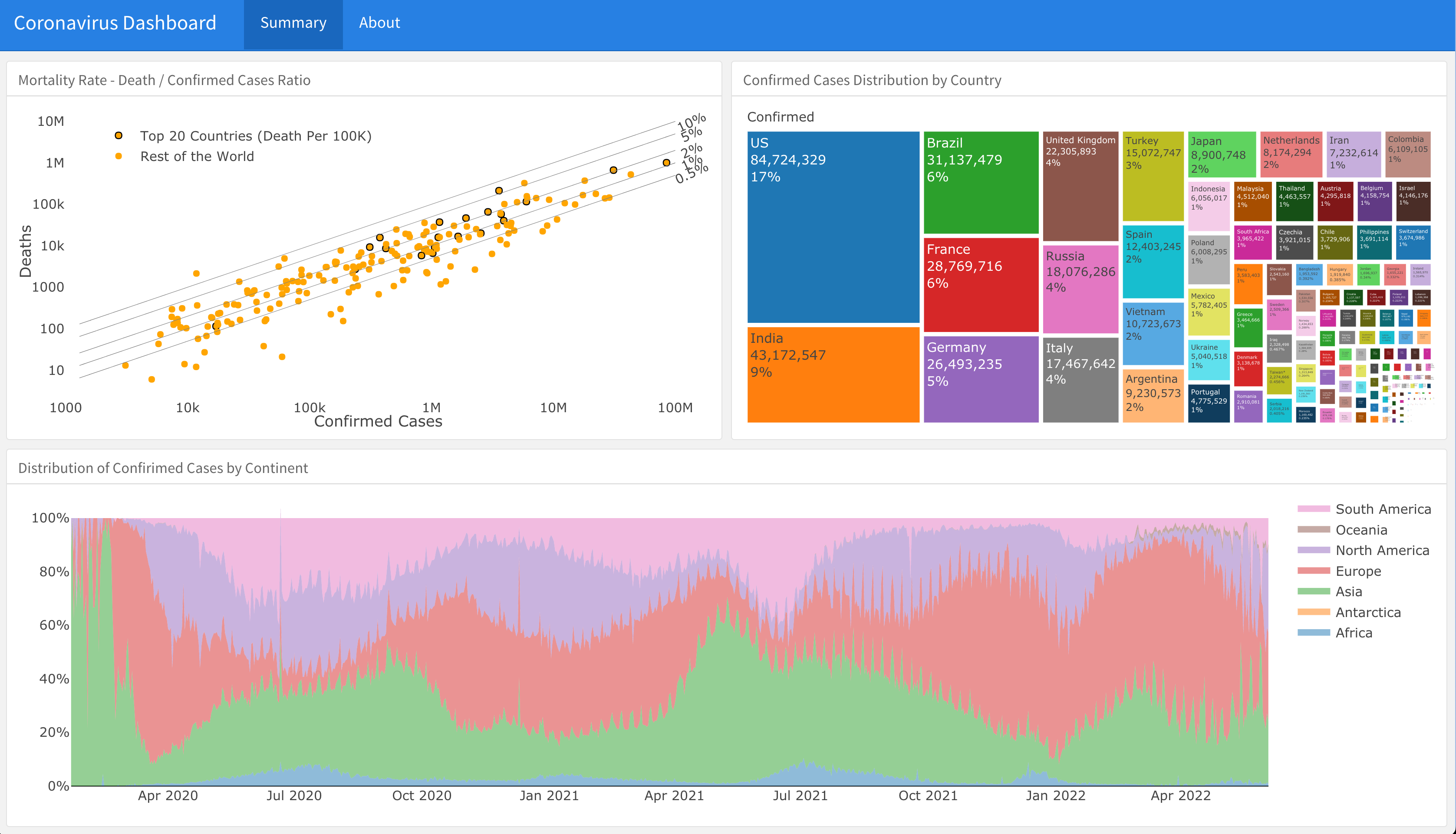
#> 6   124 Alberta, Canada    4413146  North America             NA

Summary of the total confrimed cases by country (top 20):

library(dplyr)

summary_df <- coronavirus %>% 
  filter(type == "confirmed") %>%
  group_by(country) %>%
  summarise(total_cases = sum(cases)) %>%
  arrange(-total_cases)

summary_df %>% head(20) 
#> # A tibble: 20 × 2
#>    country        total_cases
#>    <chr>                <int>
#>  1 US                86636306
#>  2 India             43344958
#>  3 Brazil            31890733
#>  4 France            30555038
#>  5 Germany           27573585
#>  6 United Kingdom    22751393
#>  7 Korea, South      18305783
#>  8 Russia            18137759
#>  9 Italy             18014202
#> 10 Turkey            15085742
#> 11 Spain             12613634
#> 12 Vietnam           10739855
#> 13 Argentina          9341492
#> 14 Japan              9178003
#> 15 Netherlands        8247488
#> 16 Australia          7919844
#> 17 Iran               7235440
#> 18 Colombia           6131657
#> 19 Indonesia          6072918
#> 20 Poland             6011984

Summary of new cases during the past 24 hours by country and type (as of 2022-06-22):

library(tidyr)

coronavirus %>% 
  filter(date == max(date)) %>%
  select(country, type, cases) %>%
  group_by(country, type) %>%
  summarise(total_cases = sum(cases)) %>%
  pivot_wider(names_from = type,
              values_from = total_cases) %>%
  arrange(-confirmed)
#> # A tibble: 199 × 4
#> # Groups:   country [199]
#>    country        confirmed death recovery
#>    <chr>              <int> <int>    <int>
#>  1 US                184074   860        0
#>  2 Germany           119360    98        0
#>  3 France             78123    66        0
#>  4 Brazil             71906   140        0
#>  5 Italy              54873    50        0
#>  6 Taiwan*            52218   171        0
#>  7 United Kingdom     33406    77        0
#>  8 Australia          32034    52        0
#>  9 Japan              17263    15        0
#> 10 Portugal           15372    21        0
#> # … with 189 more rows

Plotting daily confirmed and death cases in Brazil:

library(plotly)

coronavirus %>% 
  group_by(type, date) %>%
  summarise(total_cases = sum(cases)) %>%
  pivot_wider(names_from = type, values_from = total_cases) %>%
  arrange(date) %>%
  mutate(active = confirmed - death - recovery) %>%
  mutate(active_total = cumsum(active),
                recovered_total = cumsum(recovery),
                death_total = cumsum(death)) %>%
  plot_ly(x = ~ date,
                  y = ~ active_total,
                  name = 'Active', 
                  fillcolor = '#1f77b4',
                  type = 'scatter',
                  mode = 'none', 
                  stackgroup = 'one') %>%
  add_trace(y = ~ death_total, 
             name = "Death",
             fillcolor = '#E41317') %>%
  add_trace(y = ~recovered_total, 
            name = 'Recovered', 
            fillcolor = 'forestgreen') %>%
  layout(title = "Distribution of Covid19 Cases Worldwide",
         legend = list(x = 0.1, y = 0.9),
         yaxis = list(title = "Number of Cases"),
         xaxis = list(title = "Source: Johns Hopkins University Center for Systems Science and Engineering"))

Plot the confirmed cases distribution by counrty with treemap plot:

conf_df <- coronavirus %>% 
  filter(type == "confirmed") %>%
  group_by(country) %>%
  summarise(total_cases = sum(cases)) %>%
  arrange(-total_cases) %>%
  mutate(parents = "Confirmed") %>%
  ungroup() 
  
  plot_ly(data = conf_df,
          type= "treemap",
          values = ~total_cases,
          labels= ~ country,
          parents=  ~parents,
          domain = list(column=0),
          name = "Confirmed",
          textinfo="label+value+percent parent")

data(covid19_vaccine)

head(covid19_vaccine)
#>   country_region       date doses_admin people_partially_vaccinated
#> 1         Canada 2020-12-14           5                           0
#> 2          World 2020-12-14           5                           0
#> 3         Canada 2020-12-15         723                           0
#> 4          China 2020-12-15     1500000                           0
#> 5         Russia 2020-12-15       28500                       28500
#> 6          World 2020-12-15     1529223                       28500
#>   people_fully_vaccinated report_date_string uid province_state iso2 iso3 code3
#> 1                       0         2020-12-14 124           <NA>   CA  CAN   124
#> 2                       0         2020-12-14  NA           <NA> <NA> <NA>    NA
#> 3                       0         2020-12-15 124           <NA>   CA  CAN   124
#> 4                       0         2020-12-15 156           <NA>   CN  CHN   156
#> 5                       0         2020-12-15 643           <NA>   RU  RUS   643
#> 6                       0         2020-12-15  NA           <NA> <NA> <NA>    NA
#>   fips      lat     long combined_key population continent_name continent_code
#> 1 <NA> 60.00000 -95.0000       Canada   37855702  North America             NA
#> 2 <NA>       NA       NA         <NA>         NA           <NA>           <NA>
#> 3 <NA> 60.00000 -95.0000       Canada   37855702  North America             NA
#> 4 <NA> 35.86170 104.1954        China 1404676330           Asia             AS
#> 5 <NA> 61.52401 105.3188       Russia  145934460         Europe             EU
#> 6 <NA>       NA       NA         <NA>         NA           <NA>           <NA>

Plot the top 20 vaccinated countries:

covid19_vaccine %>% 
  filter(date == max(date),
         !is.na(population)) %>% 
  mutate(fully_vaccinated_ratio = people_fully_vaccinated / population) %>%
  arrange(- fully_vaccinated_ratio) %>%
  slice_head(n = 20) %>%
  arrange(fully_vaccinated_ratio) %>%
  mutate(country = factor(country_region, levels = country_region)) %>%
  plot_ly(y = ~ country,
          x = ~ round(100 * fully_vaccinated_ratio, 2),
          text = ~ paste(round(100 * fully_vaccinated_ratio, 1), "%"),
          textposition = 'auto',
          orientation = "h",
          type = "bar") %>%
  layout(title = "Percentage of Fully Vaccineted Population - Top 20 Countries",
         yaxis = list(title = ""),
         xaxis = list(title = "Source: Johns Hopkins Centers for Civic Impact",
                      ticksuffix = "%"))